Bias-Variance Tradeoff Explained with Visual Examples

Contents

Figure 1: Two ways to be wrong — too rigid, or too eager

400 models, measured bias², variance and noise, plus figures you can see

Every machine learning model makes two kinds of mistakes. It can be too stubborn to learn the real pattern, or too eager and learn the noise too. Fix one, and the other gets worse.

That tension is the bias-variance tradeoff, and most explanations stay abstract. So I ran an experiment you can see: 400 models, each trained on a fresh sample of data, with measured numbers and three figures. Everything below comes from a script run with NumPy and matplotlib.

The Setup

I created data from a known curve, y = sin(2πx), and added random noise (standard deviation 0.3). Each training set has just 20 points. Then I fit polynomials of degree 1 through 15 to 400 different training sets, redrawing the noise each time.

Why 400 sets? Bias and variance describe what happens across many possible training sets, not in one. A single model can't show you either. A crowd of models can.

One technical note: I held the x positions fixed and redrew only the noise. That's the textbook setup, and it keeps the numbers well-behaved.

Three Kinds of Error

Any model's expected error on new data splits into three parts:

• Bias²: how far the average model is from the truth. High bias means the model is too simple, so it misses the pattern no matter how much data it sees.
• Variance: how much the model changes from one training set to another. High variance means it chases noise in whatever sample it got.
• Irreducible noise: randomness in the data itself. Here it's 0.3² = 0.09. No model beats it.

The formula is just addition: expected error = bias² + variance + noise. The script checks this: for every degree, the sum matched the directly measured test error to within a few percent.

See It: Three Models, Three Personalities

Figure 1 shows 40 of the 400 fitted models in each panel, with the true curve dashed and the average fit in bold blue.

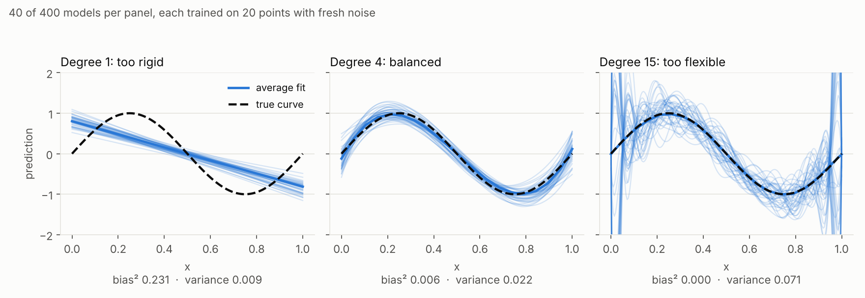
• Degree 1: too rigid. Every model is a nearly identical straight line, and every one misses the sine wave. That's high bias (bias² 0.231) and low variance (0.009). Even more data won't help, as we'll see.
• Degree 4: balanced. The models hug the true curve, with only a small fan of disagreement. Bias² is 0.006 and variance is 0.022.
• Degree 15: too flexible. Here's the mess. The average model (bold) sits right on the true curve, so bias² is essentially 0.000. But individual models thrash wildly, especially near the edges. Variance is 0.071, about eight times the degree-1 value. Each model memorized its own sample's noise.

FYI, the average is right and the individual models are wrong. That's exactly what high variance looks like.

The Tradeoff in One Chart

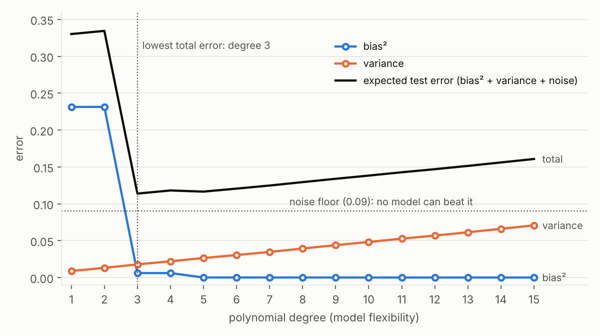
Figure 2 plots all three components against model flexibility:

Degree	Bias²	Variance	Expected test error
1	0.231	0.009	0.330
2	0.231	0.013	0.334
3	0.006	0.018	0.114
4	0.006	0.022	0.118
8	0.000	0.039	0.129
15	0.000	0.071	0.161

Read it left to right:

• Bias² collapses. From degree 2 to 3, it falls from 0.231 to 0.006. (It stays put from 1 to 2 because a sine wave is symmetric, so a squared term adds nothing here. Cute detail, not a general rule.)
• Variance climbs steadily. Each extra parameter adds a little.
• Total error is U-shaped, with its minimum at degree 3.

Variance isn't magic, either. For plain least squares it follows a formula: noise variance × number of parameters ÷ number of points. For degree 15 that predicts 0.0720, and I measured 0.0707. For degree 3 it predicts 0.0180, and I measured 0.0178. The simulation agrees with the math.

Training Error Lies

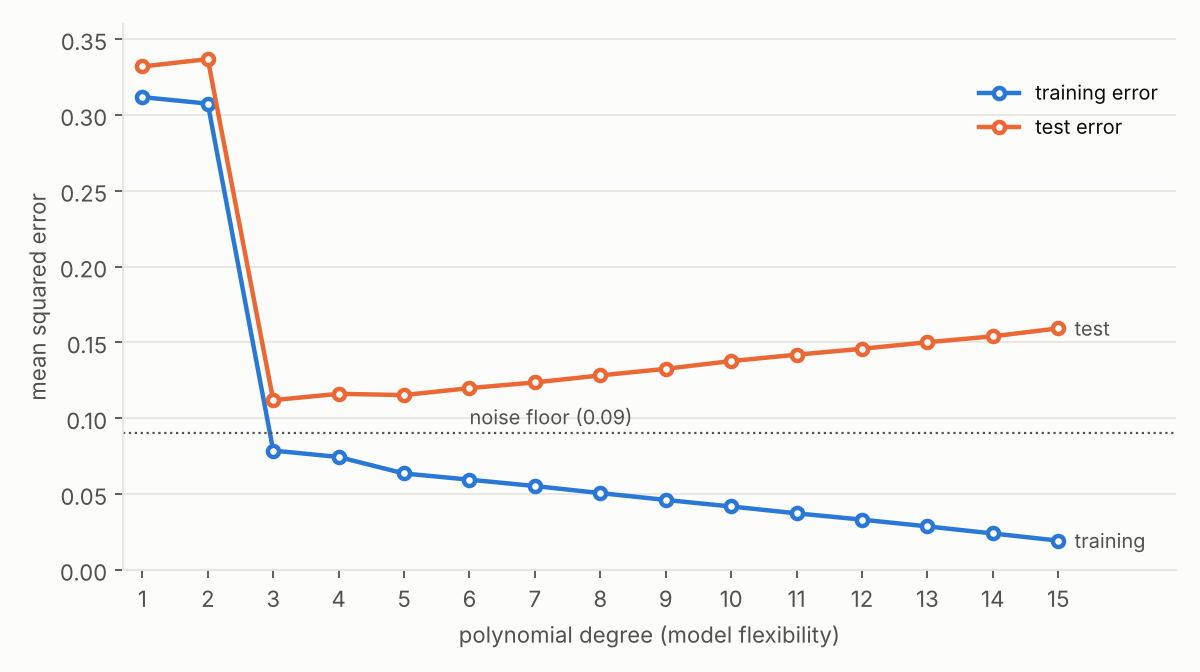
Figure 3 shows what you'd see if you only checked training performance:

Degree	Training error	Test error
1	0.312	0.332
3	0.079	0.112
8	0.051	0.128
15	0.019	0.159

Training error keeps falling forever. At degree 15 it hits 0.019, far below the 0.09 noise floor, which should be impossible for an honest model. It's fitting noise. Meanwhile test error bottoms out at degree 3 and then drifts up. That growing gap between the two curves is your overfitting alarm. In my experience it's the single most useful diagnostic in machine learning.

The U-shape here is mild: 0.112 at the best point and 0.159 at the worst. That's because my setup is gentle. In an earlier run I used random x positions with 30 points, and degree-15 test error exploded to hundreds of millions, because high-degree polynomials go wild between gaps in the data. Real overfitting can be far uglier than the chart suggests.

Which Problem Do You Have?

Diagnose before you treat:

Symptom	Likely problem
High training error, test error about the same	High bias (underfitting)
Low training error, much higher test error	High variance (overfitting)
Both low and close	Good fit

Fixes: More Data

I tested whether more data helps each problem:

Model	Points per set	Bias²	Variance	Test error
Degree 15	20	0.0000	0.0707	0.1593
Degree 15	100	0.0000	0.0140	0.1036
Degree 15	400	0.0000	0.0035	0.0935
Degree 1	20	0.2313	0.0088	0.3320
Degree 1	400	0.1978	0.0004	0.2883

More data crushes variance. The degree-15 model's variance fell twentyfold, and its test error approached the 0.09 noise floor. But the degree-1 model barely improved: its bias² stayed near 0.2, so test error was still 0.288. More data can't fix a model that's too simple. (The small bias change between 20 and 400 points comes from measuring at different x positions, not from learning anything new.)

Fixes: Regularization

Regularization trades a little bias for less variance. I added a ridge penalty to the degree-15 model:

Penalty (alpha)	Bias²	Variance	Test error
0	0.0000	0.0707	0.1593
0.1	0.0001	0.0623	0.1506
1	0.0031	0.0525	0.1445
10	0.0966	0.0191	0.2069

A little penalty helps: at alpha = 1, variance dropped and bias barely rose, so test error improved. Push too far, at alpha = 10, and bias takes over. That's the tradeoff in miniature. The honest caveat: the gain is modest here (0.159 to 0.145), and a simple degree-3 model still beat every regularized degree-15 version I tried (0.112). Sometimes the best fix is a simpler model. Ensembles like random forests attack the same problem from the other side — averaging many high-variance models to cancel variance without adding bias.

A Practical Playbook

1. Underfitting? Add features, use a more flexible model, or reduce regularization.
2. Overfitting? Get more data, simplify the model, add regularization, or stop training earlier.
3. Always compare training and validation error, never training alone — the setup from the cross-validation guide in this series.
4. Don't chase zero. The noise floor means some error is permanent.

For where this fits in the wider landscape of models, the algorithms guide maps the terrain.

Common Pitfalls

• Judging a model on training error alone, which only ever goes down as flexibility rises.
• Assuming more data fixes everything — it can't touch bias.
• Regularizing blindly until bias quietly takes over.
• Comparing train and test on one split and calling it a diagnosis.
• Treating the noise floor as a failure — some error is irreducible.
• Picking model complexity by reputation instead of the U-shaped curve.
• Ignoring the gap between the curves — it's the overfitting signal.
• Assuming the tradeoff is theoretical — the tables above measured it directly.

Unlock AI That Actually Works

Get lifetime access to GPT-6 Astra, Claude Fable 5.1, Gemini 3.5, Grok 4.5, and more — all in one platform. Build websites, apps, videos, content, and digital products from a single command. No monthly fees. No tool-hopping.

Click here to get GPTAstra Max now — one-time payment, lifetime access.

Frequently Asked Questions

What is the bias-variance tradeoff?

Expected error on new data splits into three additive parts: bias² (how far the average model is from the truth), variance (how much the model changes across different training sets), and irreducible noise (randomness in the data itself). Simple models have high bias and low variance, flexible models have low bias and high variance, and total error is U-shaped with its minimum somewhere in between — degree 3 in the polynomial experiment, at 0.114 expected test error.

How do I tell whether my model has high bias or high variance?

Compare training error with test error. If both are high and close together, the model is too simple — high bias, underfitting. If training error is low but test error is much higher, the model memorized noise — high variance, overfitting. In the experiments, degree-15 polynomials hit a training error of 0.019 (below the 0.09 noise floor) while test error sat at 0.159, the classic overfitting alarm.

Does more data fix overfitting?

Yes, for variance — and only for variance. Growing the training set from 20 to 400 points cut the degree-15 model's variance twentyfold (0.0707 to 0.0035) and pulled test error down to 0.0935, near the noise floor. But the degree-1 model barely moved: its bias² stayed around 0.2 and test error was still 0.288. More data can't fix a model that's too simple to capture the pattern.

Does regularization fix overfitting?

Partially, and it's a trade. A ridge penalty on the degree-15 model at alpha=1 cut variance from 0.0707 to 0.0525 while bias² rose only to 0.0031, improving test error to 0.1445. Pushed to alpha=10 the bias took over (0.0966) and test error worsened to 0.2069. Regularization trades a little bias for less variance — and in this experiment a plain degree-3 model (0.112) still beat every regularized degree-15 version.

Wrapping This Up

Bias is being wrong in a consistent way. Variance is being wrong differently every time. Total error is bias² plus variance plus noise, and the best model sits where the first two balance. In my experiment that was degree 3, and you could see why in the figures.

Next step: grab the script and change the settings. Raise the noise, shrink the training set, or swap in a different curve. Then watch where the U-shape's bottom moves.

Related Articles

• Linear Regression in Python: From Scratch to Scikit-Learn
• Random Forest Algorithm Explained with Python Code
• Machine Learning Algorithms Explained: Complete Beginner's Guide
• Scikit-learn Cross-Validation: Master K-Fold Testing