 Buy me a coffee


Contents
Figure 1: Maximum Likelihood Estimation Explained: From Coin Flips to Logistic Regression — one principle, from a coin on a table to the solver inside every classifier you train
You flip a coin ten times. Seven heads, three tails. What is your best guess for the probability of heads?
If you said "0.7", you just did maximum likelihood estimation without knowing it. MLE is the engine under logistic regression, the reason your spam filter works, and the principle behind most models you have trained.
I once watched a room of PhD students freeze when a professor asked, "So why do we maximise the likelihood again?" The silence was painful. This article is the answer I wish someone had given that room.
The Core Idea: What Makes Your Data Most Probable?
We observe data, but never the process that generated it. We see seven heads; we do not see the coin's bias. MLE asks one question:
Which parameter value makes the observed data most likely to have happened?
Not "which parameter is true" — that is unknowable. Not "which parameter minimises error" — that is a different philosophy with different answers. Which parameter makes this specific dataset most probable?
The coin flip example
A coin flip is a Bernoulli trial with probability of heads p. We saw 7 heads and 3 tails in 10 flips, so the likelihood is:
L(p) = p⁷(1 − p)³
Maximising a product is awkward, so take the log — same maximum, easier algebra:
ℓ(p) = 7 log(p) + 3 log(1 − p)
Differentiate and set to zero:
7/p − 3/(1 − p) = 0 → p = 0.7
The MLE is exactly the sample proportion. That is not a coincidence; it is a property of exponential families, which we get to shortly.
Why "likelihood" not "probability"?
Probability describes outcomes given a parameter; likelihood describes parameters given an outcome.
P(data | parameter)— probability, forwardL(parameter | data)— likelihood, backward
It is the same mathematical expression with a different interpretation. The parameter is fixed but unknown. The data is what varies across hypothetical repetitions.
This distinction is where most textbooks lose people. Likelihood is a function of the parameter with the data held fixed — that is the whole idea, and it explains why likelihoods do not integrate to one over the parameter.
From Coins to Continuous: The Normal Distribution
Coin flips are discrete. Heights are not: 170, 175, 168, 182, 177 cm. Assume a normal distribution with unknown mean μ and known variance σ².
The log-likelihood is:
ℓ(μ) = −(n/2) log(2πσ²) − (1/2σ²) ∑(xᵢ − μ)²
The first term is constant, so maximising the log-likelihood is the same as minimising the sum of squared deviations. The MLE for μ is the sample mean.
Least squares is maximum likelihood under normality. Two apparently different traditions, one derivation.
What if variance is unknown too?
Now both parameters are free. The log-likelihood is:
ℓ(μ, σ²) = −(n/2) log(2π) − (n/2) log(σ²) − (1/2σ²) ∑(xᵢ − μ)²
The partial derivative with respect to μ gives the sample mean again. The derivative with respect to σ² gives:
σ̂² = (1/n) ∑(xᵢ − x̄)²
Notice the n, not n − 1. The MLE for variance is biased downward, though consistent, and the unbiased version divides by n − 1. The bias vanishes asymptotically but matters at small samples, which is why every statistics course argues about it.
The Exponential Family: Why MLE Is So Tidy
Ever notice how many distributions produce clean closed-form MLEs? Bernoulli, normal, Poisson, exponential, gamma, beta — all exponential family distributions.
A distribution is in the exponential family if its density can be written:
f(x | θ) = h(x) exp{ η(θ)ᵀ T(x) − A(θ) }
η(θ)— the natural parameterT(x)— the sufficient statisticA(θ)— the log partition functionh(x)— the base measure
The magic is that the MLE of the expected sufficient statistic is just the sample average of T(x). Since E[T(X)] = ∇A(η), you set the sample average equal to the theoretical expectation and solve.
That single fact explains a lot of familiar results:
- Bernoulli:
E[X] = p, so the MLE is the sample proportion - Poisson:
E[X] = λ, so the MLE is the sample mean - Normal:
E[X] = μandE[X²] = μ² + σ², so the MLEs are the sample moments
The exponential family is MLE's comfort zone. Step outside it — logistic regression, Cox models, mixture models — and you need numerical optimisation [1].
The General Recipe: How to MLE Anything
Every MLE problem follows the same five steps:
- Write the likelihood for your model, then take the log.
- Differentiate with respect to each parameter.
- Set the derivatives to zero — these are the score equations.
- Solve for the parameters.
- Verify it is a maximum — second derivative, or the Hessian, should be negative definite.
Sometimes step 4 is algebra (normal mean, Bernoulli p). Sometimes it needs a solver (logistic regression, Poisson regression, anything with a link function).
The score function
The derivative of the log-likelihood is the score function, and setting it to zero gives the score equations:
U(θ) = ∂ℓ(θ)/∂θ = 0
The score has mean zero at the true parameter, and its variance is the Fisher information. That is the bridge from estimation to uncertainty.
Fisher information: the curvature of knowledge
The Fisher information is:
I(θ) = −E[∂²ℓ/∂θ∂θᵀ] = Var[U(θ)]
It measures how sharply the log-likelihood curves at its peak, which is how much information the data carries about the parameter. High curvature means a precise estimate.
For a normal mean with known variance, I(μ) = n/σ² — more data or less noise gives more information, exactly as intuition says.
The asymptotic variance of the MLE is I(θ)⁻¹, which is the Cramér-Rao lower bound. No consistent estimator does better in the limit.
Logistic Regression: MLE's Greatest Hit
This is where MLE stops being a textbook exercise. Logistic regression models:
P(Y = 1 | X) = 1 / (1 + exp(−Xβ))
There is no closed-form solution. The likelihood is a product of Bernoulli probabilities with pᵢ = σ(xᵢᵀβ), so the log-likelihood is:
ℓ(β) = ∑ [ yᵢ log(pᵢ) + (1 − yᵢ) log(1 − pᵢ) ]
The score equations are compact and famous:
Xᵀ(y − p) = 0
You solve them iteratively — with Newton-Raphson, which becomes iteratively reweighted least squares, or with a quasi-Newton method such as L-BFGS [3].
Inside IRLS: the Newton-Raphson connection
Newton-Raphson updates take the form:
β⁽ᵏ⁺¹⁾ = β⁽ᵏ⁾ − H⁻¹U
For logistic regression, the score is U = Xᵀ(y − p) and the Hessian is H = −XᵀWX with W = diag(pᵢ(1 − pᵢ)). Substituting gives:
β⁽ᵏ⁺¹⁾ = (XᵀWX)⁻¹ XᵀWz, where z = Xβ⁽ᵏ⁾ + W⁻¹(y − p)
That is exactly weighted least squares on the working response z with weights W. Each iteration solves a weighted regression problem, and the weights are largest where p = 0.5.
So observations near the decision boundary get the most weight, because those are the ones that still carry information about where the boundary should be. Points already confidently classified barely move it [2].
Why Not Least Squares?
You could fit a classifier by regressing the labels on the features, but the result misbehaves:
- Predicted probabilities leave
[0, 1], because a straight line has no reason to respect the range. - The variance depends on the mean — Bernoulli data is heteroscedastic by construction — so ordinary least squares weights observations incorrectly.
- MLE weights each observation by its information content, which is the correct weighting for binomial data.
MLE is not an arbitrary choice here. It is the estimator implied by the likelihood you already assumed when you wrote the model down.
Properties That Make MLE Special
- Consistency. As
n → ∞, the MLE converges to the true parameter. - Asymptotic normality.
√n(θ̂ − θ) → N(0, I(θ)⁻¹), which is what makes confidence intervals and Wald tests valid for large samples. - Invariance. If
θ̂is the MLE ofθ, theng(θ̂)is the MLE ofg(θ). Estimate first or transform first — same answer. - Efficiency. The MLE attains the Cramér-Rao bound asymptotically, so no consistent estimator has smaller asymptotic variance.
That is a remarkable list for one principle, and it is why MLE became the default across statistics and machine learning.
When MLE Goes Wrong
Fair warning: MLE is not magic.
- Small samples. The asymptotic guarantees vanish, and the bias can be substantial — especially for variance parameters.
- Separation. Perfect prediction in logistic regression drives coefficients to infinity. Firth's penalised MLE fixes it [4].
- Misspecification. The wrong likelihood gives wrong answers with confident standard errors. Quasi-likelihood and sandwich estimators help.
- Boundary problems. Variance estimates can hit zero, which is where REML beats MLE for variance components.
- Multimodality. Mixture models and hidden Markov models have many local maxima, so you need the EM algorithm, multiple starts, or both.
The separation problem in detail
Complete separation means some linear combination of predictors perfectly predicts the outcome. The likelihood then keeps increasing as the coefficients grow, so no finite MLE exists and the software either warns you or returns enormous coefficients with enormous standard errors.
Quasi-complete separation is the same disease with partial overlap: the MLE exists, but it is huge and unstable.
Firth's penalty adds ½ log|I(β)| to the log-likelihood, which shrinks coefficients toward zero and removes the first-order bias. It is now standard practice in epidemiology and in any analysis with rare events, where rare-event bias correction is the close cousin of the same idea [4][5].
The Bayesian Elephant in the Room
MLE gives a point estimate; Bayesians want a posterior distribution. The Bayesian objection is essentially: "You are maximising the likelihood? Cute. I am integrating over the prior."
MAP estimation is MLE plus a prior. Add the log-prior to the log-likelihood and maximise. That single change explains two familiar estimators:
- Ridge regression is MAP with a Gaussian prior.
- Lasso is MAP with a Laplace prior, which is why it produces zeros — the geometry I broke down in why lasso gives sparse solutions.
Frequentist MLE is Bayesian MAP with a flat prior. Two philosophies, the same arithmetic, different interpretations of what the answer means.
Laplace approximation: Bayes meets MLE
For large n, the posterior is approximately normal:
θ | data ≈ N(θ̂, I(θ̂)⁻¹)
The MLE is the posterior mode, and the posterior covariance is the inverse Fisher information. Asymptotically, frequentists and Bayesians agree; the arguments that remain are about small samples and priors.
Practical Tips From the Trenches
- Always use the log-likelihood. Products become sums, underflow disappears, gradients are cleaner.
- Check your gradients numerically. Analytical and finite-difference gradients should agree to about
1e-6. If they do not, your derivative is wrong, and this check saves weeks. - Use profile likelihood for confidence intervals. Wald intervals (
θ̂ ± 1.96 SE) are garbage for small samples or skewed likelihoods; profile intervals respect the actual shape. - Start from good values. Newton-Raphson diverges from bad starts, so initialise with method of moments, a simple regression, or a coarse grid.
- Monitor three convergence criteria — parameter change, gradient norm, and log-likelihood change. One is not enough.
Profile likelihood works like this: fix θⱼ, maximise over everything else, and repeat across a grid. The 95% interval is where the log-likelihood has dropped by 1.92 from its maximum — that is ½ χ²₁ at 95%.
Common Pitfalls
- Summing likelihoods. Likelihoods multiply, log-likelihoods add. Mixing them up produces nonsense.
- Forgetting the
nversusn − 1. The MLE variance is biased; report which one you used. - Trusting a converged solver. Convergence to a saddle point or a boundary is still "converged" as far as the optimiser is concerned.
- Reporting Wald intervals for a skewed likelihood. Profile likelihood is the honest option.
- Ignoring separation warnings. Enormous coefficients with enormous standard errors are a symptom, not a result.
- Comparing log-likelihoods across transformed responses. Change
ytolog(y)and you need the Jacobian adjustment before the numbers are comparable. - Assuming MLE is unbiased. It is asymptotically unbiased, which is a different sentence.
- Using MLE for variance components when REML exists. The bias is real at small group counts.
Most of these are the same mistake: treating an asymptotic guarantee as a promise about your actual sample.
Best Book to Read
| Cover | Book | Description | Get it |
|---|---|---|---|
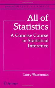 |
All of Statistics | a compact graduate course covering point estimation, the score function, Fisher information, asymptotics, and the bootstrap in about 450 pages. | View on Amazon |
As an Amazon Associate I earn from qualifying purchases. Links on this page are affiliate links, and I may earn a commission at no extra cost to you.
Read the point-estimation and asymptotics chapters first. Wasserman keeps the proofs short and the intuition sharp, which is exactly the balance this topic needs. The PDF is free on the author's site.
Wrapping Up
Maximum likelihood estimation is not a technique; it is a principle. Choose the parameter that makes your observed data most probable.
From coin flips (p = 0.7) to logistic regression (IRLS iterations) to the asymptotic normality behind your confidence intervals, MLE is the thread connecting all of it. Consistent, asymptotically normal, efficient, invariant — the greatest-hits album of statistical properties.
Next time you fit a model, remember you are not minimising error. You are maximising the probability that this exact dataset happened. That is a genuinely different way to see the world, and it is the mental model that makes the rest of statistics legible — the same reason I argued for intuition before proofs in ML maths.
Now go maximise some likelihoods. And maybe flip a coin while you are at it.
Frequently Asked Questions
What is maximum likelihood estimation in simple terms?
MLE picks the parameter value that makes the data you actually observed most probable. Flip a coin ten times and see seven heads, and the most likely bias is 0.7. You are not finding the true parameter, because that is unknowable — only the value that best explains this dataset.
Why do we take the log of the likelihood?
Because the likelihood is a product of probabilities, and products underflow to zero for large samples. The log turns products into sums, keeps the same maximum, and makes derivatives far simpler. Every optimizer works with the log-likelihood for that reason.
Is maximum likelihood the same as least squares?
Only when you assume Gaussian noise with constant variance. Under that assumption, maximising the normal likelihood is identical to minimising the sum of squared residuals. Change the noise model and the two diverge, which is why logistic regression uses log-loss instead of squared error.
Why does logistic regression have no closed-form solution?
The score equations are non-linear in the coefficients, so no algebraic rearrangement isolates beta. You solve them iteratively with Newton-Raphson, which becomes iteratively reweighted least squares, or with a quasi-Newton solver such as L-BFGS.
What is the difference between MLE and MAP?
MAP adds a prior to the likelihood before maximising, so the estimate is pulled toward prior belief. MLE is MAP with a flat prior. Ridge regression is MAP with a Gaussian prior and lasso is MAP with a Laplace prior, which is why they shrink coefficients.
Sources
[1]Wasserman, All of Statistics — point estimation, exponential families, Fisher information, and asymptotics; free PDF: stat.cmu.edu/~larry/all-of-statistics[2]statsmodels, Generalized Linear Models — the IRLS implementation and its convergence behaviour: statsmodels.org/stable/glm.html[3]scikit-learn, Logistic regression — solvers, regularisation, and the log-loss formulation: scikit-learn.org/stable/modules/linear_model.html[4]Firth, Bias reduction of maximum likelihood estimates (1993) — the penalised likelihood that fixes separation: doi.org/10.1093/biomet/80.1.27[5]King and Zeng, Logistic Regression in Rare Events Data — why separation and rare events break the usual estimates: gking.harvard.edu


 Get Free Course Notes →