 Buy me a coffee


Contents
Figure 1: How to Tell If One Model Is Really Better: Bootstrap Confidence Intervals and Paired Tests — two runners a fraction of a second apart: the question is not who finished first, but whether the gap is larger than the wobble in the clock
Model A scores 91.2% and model B scores 90.8%. You ship A, and your teammate asks whether the gap means anything. Do you have an answer?
Most of us have shrugged at that question at least once. A single test-set score is a point estimate with no error bar, and a ranking without an error bar is not evidence. This article turns "A scored higher" into "A is better, and here is how sure I am" — using the bootstrap, McNemar's test, and the 5×2 cross-validation test.
Why a Single Score Lies
A test set is a sample. Draw a different sample of the same size from the same population and you get a different score; the ranking of two close models can flip. The smaller the test set, the bigger the wobble.
Put numbers on it. A classifier makes 12 mistakes on 40 test examples, so its error rate is 30%. The textbook 95% interval — the normal approximation, or Wald interval — runs from 15.8% to 44.2%:
0.30 ± 1.96 × √(0.30 × 0.70 / 40)
The Wald interval is the one most textbooks show, and it is not the best at this sample size. The Wilson interval gives 18.1% to 45.4%, and the bootstrap percentile lands in the same neighbourhood. The exact endpoints matter less than the width.
That is a 28-point window around a single number. Any gap much smaller than that window is hard to defend with this test set.
But do not compare two intervals by eye. Both models are scored on the same examples, so their errors are correlated: the hard images trip up both models, and the easy ones are easy for both. Comparing separate intervals throws that pairing away, which is the mistake the paired design fixes below.
The question changes. Instead of "which score is higher?", ask "how big is the difference, and could noise explain it?"
Step 1: Put an Interval Around Your Metric
The bootstrap gives you an interval for almost any metric, including ones with no tidy formula, such as F1, AUC, or BLEU. The recipe is four lines:
- Resample the test set with replacement, keeping the same size.
- Compute the metric on that resample.
- Repeat a thousand times or more.
- Take the 2.5th and 97.5th percentiles as the 95% interval.
The spread shows how much the score depends on which examples happened to land in the test set. You do not need a distributional formula, which is why the method works for metrics that statisticians never derived a closed form for.
It is not assumption-free, though. The bootstrap treats the test set as a stand-in for the population, so it cannot fix a biased sample, and it assumes the examples are exchangeable. If your data are grouped — many images per patient, many rows per user — resample whole groups, not rows. Otherwise the interval comes out too narrow.
Percentile Is Not the Best Interval
The percentile recipe above is what most tutorials show, and it is not the best default. Percentile intervals can under-cover for small samples and skewed metrics, because they do not correct for bias or for how fast the statistic's standard error changes with the parameter.
BCa — bias-corrected and accelerated — is the better choice [1][4]. It adjusts the percentile endpoints for bias and skew, and it is one keyword away:
from scipy.stats import bootstrap

res = bootstrap(
    (y_test, preds_a),
    lambda y, p: (y == p).mean(),
    paired=True, n_resamples=10_000,
    confidence_level=0.95, method="BCa",
)
Use the percentile interval when you want the simplest thing that works, and BCa when the metric is skewed or the sample is small. For a 500-example test set and accuracy, the two usually agree closely; for F1 on a rare class, they can differ meaningfully.
Step 2: Compare Two Models With a Paired Bootstrap
You could bootstrap each model separately and see whether the intervals overlap. Don't. Separate intervals ignore the correlation between the two models and give you a muddled answer — usually a conservative one, sometimes an incoherent one.
The paired bootstrap fixes it. Resample the test indices once, score both models on that same resample, and record the difference:
Δ* = metric(A on resample) − metric(B on resample)
Repeat many times. If the 95% interval of Δ* excludes zero, you have evidence that one model beats the other.
import numpy as np

def paired_bootstrap(y_true, pred_a, pred_b, metric, n_boot=5000, seed=0):
    rng = np.random.default_rng(seed)
    n = len(y_true)
    diffs = np.empty(n_boot)
    for i in range(n_boot):
        idx = rng.integers(0, n, n)          # same indices for both models
        diffs[i] = metric(y_true[idx], pred_a[idx]) - metric(y_true[idx], pred_b[idx])
    lo, hi = np.percentile(diffs, [2.5, 97.5])
    return diffs.mean(), (lo, hi)

acc = lambda y, p: (y == p).mean()
mean_diff, ci = paired_bootstrap(y_test, preds_a, preds_b, acc)
observed = acc(y_test, preds_a) - acc(y_test, preds_b)

print(f"observed A - B: {observed:+.4f}")
print(f"bootstrap mean: {mean_diff:+.4f}, 95% CI {ci[0]:+.4f} to {ci[1]:+.4f}")
Read the output like this.
[+0.002, +0.019]says A probably beats B, though the gap could be tiny.[−0.008, +0.017]says you cannot tell them apart at this sample size.
Two details matter more than they look.
First, report the observed difference, not the bootstrap mean. The function returns the average of the resampled differences; that is a resampling artifact, not a new measurement. The point estimate is acc(y_test, preds_a) - acc(y_test, preds_b) on the original test set, and the interval is the uncertainty around it.
Second, the interval and the p-value are different calculations. A quick bootstrap p-value is the fraction of resamples on the wrong side of zero, doubled for a two-sided test. The interval is the more informative object; use the p-value when a reviewer asks for one, but do not pretend the two are interchangeable.
McNemar's Test: Focus on Disagreements
For two classifiers on a single test set, McNemar's test is the classic alternative. It ignores the examples where both models agree — both right or both wrong — because those carry no information about which model is better. It counts only the disagreements.
| B correct | B wrong | |
|---|---|---|
| A correct | both right | b |
| A wrong | c |
both wrong |
Here b is "A right, B wrong" and c is "A wrong, B right". If the models perform equally, b and c should be roughly equal. McNemar's test asks whether they differ more than chance allows.
The statistic is:
χ² = (b − c)² / (b + c)
With a continuity correction, which is the more common variant:
χ² = (|b − c| − 1)² / (b + c)
It follows a chi-squared distribution with one degree of freedom, so a value above 3.84 rejects the "same error rate" hypothesis at the 95% level [3].
from mlxtend.evaluate import mcnemar_table, mcnemar

tb = mcnemar_table(y_target=y_test, y_model1=preds_a, y_model2=preds_b)
chi2, p = mcnemar(tb, corrected=True)
print(tb)
print(f"chi2={chi2:.3f}, p={p:.4f}")

# exact=True when b + c is small (rule of thumb: below 25)
With few disagreements, use the exact binomial version — exact=True — because the chi-squared approximation is poor when b + c is small. The exact test is just a two-sided binomial test on b out of b + c with probability 0.5 [3].
Report both the McNemar p-value and the paired bootstrap interval. The p-value answers "is there a difference?"; the interval answers "how big?" And report the effect size, which for accuracy is (b − c) / n — the number of extra correct classifications divided by the test size.
One distinction the draft version of this argument usually blurs: McNemar's test is not the unpaired "difference of two proportions" test that Dietterich condemns. It is the paired version, and it is the test he recommends when only one training run is possible [2].
When You Can Retrain: The 5×2 CV Test
McNemar and the bootstrap capture test-set noise, but they miss another source: training noise. Retrain the same model with a different split or seed, and you get different weights and different predictions. A single train/test split cannot see that.
Dietterich's 5×2cv paired t-test handles it. You run five replications of two-fold cross-validation. In each replication, train both models on one half and test on the other, then swap the halves. That gives ten error estimates — five per model — and the statistic is approximately t-distributed with 5 degrees of freedom [2].
For a two-sided 95% test, the critical value is 2.571. mlxtend reports a two-tailed p-value, so that is the number to compare against [5].
from mlxtend.evaluate import paired_ttest_5x2cv

t, p = paired_ttest_5x2cv(
    estimator1=model_a, estimator2=model_b,
    X=X, y=y, random_seed=0,
)
print(f"t={t:.3f}, p={p:.4f}")
Alpaydın later proposed a combined 5×2cv F test with better properties, and it is the version many papers report. Use the 5×2cv family when repeated model fitting is computationally feasible — small to medium models where training takes seconds or minutes, not days.
The payoff is real. Dietterich's simulation found the 5×2cv test had acceptable type I error and slightly more power than McNemar's test, because it directly measures variation from the choice of training set [2]. If you can afford to train ten times, it is the better experiment. If you cannot, McNemar is the honest fallback.
Tests to Avoid
Dietterich's classic study compared several tests on how often they flag a difference that does not exist — the type I error rate. Two common ones came out badly:
- A test for the difference of two proportions.
- A paired-differences t-test over several random train/test splits.
His verdict was blunt: they should never be used [2]. A paired t-test over 10-fold cross-validation fared better but still showed somewhat elevated false positive rates.
The deeper issue is independence. Many standard tests assume independent observations, and you violate that assumption when models are evaluated on the same test set or on overlapping training sets. Cross-validation folds share training data, so their scores correlate, and a naive t-test across folds overstates your confidence.
The fix is not to stop testing. It is to use a test that respects the pairing — McNemar for one test set, 5×2cv for repeated training, the paired bootstrap for everything else.
Beyond Accuracy and Single Splits
A few practical points keep you honest:
- Check more than one metric. A model may win on accuracy and lose on recall for the rare class you care about. Threshold choice changes that trade-off — how to choose a classification threshold covers the mechanics.
- Run multiple seeds. Train each model with five or ten seeds and compare the distributions. A gap smaller than seed-to-seed variation means nothing.
- Respect grouped data. If examples cluster, resample whole groups in the bootstrap. Otherwise the interval comes out too narrow.
- Do not peek. Tune hyperparameters on validation data, then touch the test set once. Tuning against the test set inflates every score, and no statistical test can undo that.
- Account for multiple comparisons. Compare twenty models and the chance of at least one false positive at
α = 0.05is about 64% —1 − 0.95²⁰. Use Holm or Bonferroni for a family-wise guarantee, or Benjamini-Hochberg if a controlled false discovery rate is acceptable. - Remember small datasets. The plain holdout gets unreliable when data are small, so lean on repeated resampling.
Different bootstrap flavours also exist. The .632 and .632+ bootstraps blend the out-of-bag error with the training error to correct the optimistic bias of resubstitution, which helps when data are scarce. They are bias-corrected point estimators of prediction error, not confidence intervals [1]. You can bootstrap their distribution, but the .632+ number itself is a single estimate.
Statistical vs Practical Significance
Here is the trap. With a huge test set, a 0.1% improvement can come out "statistically significant" and still be worthless. With a tiny test set, a real 3% improvement can look like noise.
So always report the effect size and its interval, then ask whether that gap justifies the extra cost, latency, or complexity. A 0.2-point accuracy gain that doubles inference latency is a product decision, not a statistical one.
Ever shipped a bigger model for a gain that vanished in production? An interval that hugs zero would have warned you. Offline significance is necessary but not sufficient — the production counterpart is covered in A/B testing ML models in production, where traffic, novelty effects, and guardrail metrics enter the picture.
A Quick Decision Guide
| Situation | The test to reach for |
|---|---|
| One test set, two classifiers, quick answer | McNemar's test plus a paired bootstrap |
| Metrics like F1, AUC, or BLEU | Paired bootstrap — it works with any metric |
| Cheap training, small data | 5×2cv paired t-test, plus multiple seeds |
| Expensive training | Paired bootstrap on the test set, and as many seeds as you can afford |
| Clustered data | Group-level bootstrap |
| Many models | Multiple-comparison correction, then confirm the winner on fresh data |
For the cross-validation mechanics behind the 5×2cv test, scikit-learn cross-validation covers k-fold and stratified splits. The statistical test is only as good as the splits it runs on.
Common Pitfalls
- Comparing raw scores without any interval. The gap might sit inside the noise.
- Comparing separate intervals by eye. Both models share the test set; use the paired bootstrap instead.
- Running a t-test across overlapping CV folds without correction. Dependence inflates your confidence.
- Reusing the test set for tuning. Your final estimate turns optimistic, and the interval is now centered on the wrong number.
- Declaring a tie when you simply lack data. A wide interval means "can't tell yet", not "equal".
- Ignoring seed variance. One lucky run proves little.
- Calling the .632+ bootstrap a confidence interval. It is a bias-corrected point estimate of error.
- Using the unpaired two-proportion test and calling it McNemar. The unpaired version ignores the pairing and is the one Dietterich condemns.
- Reporting the bootstrap mean as the effect size. Report the observed difference on the original test set.
- Forgetting grouped structure. Row-level resampling understates the uncertainty when examples cluster.
Best Book to Read
| Cover | Book | Description | Get it |
|---|---|---|---|
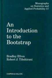 |
An Introduction to the Bootstrap | the canonical text on the bootstrap, from the percentile method through BCa, hypothesis tests, and the .632 estimators. | View on Amazon |
As an Amazon Associate I earn from qualifying purchases. Links on this page are affiliate links, and I may earn a commission at no extra cost to you.
Read the confidence-interval chapters with your own metric in hand. The book is unusually good at showing why the percentile interval can fail and what BCa changes, which is exactly the gap between the four-line recipe and an interval you can defend.
Wrapping Up
A higher score alone does not make a better model. Put a bootstrap interval around the difference, use a paired design so shared hard examples cancel out, and add McNemar's test or the 5×2cv test when the setup fits.
The three rules that matter most:
- Bootstrap the difference, not the two scores separately.
- Report the interval and the effect size, not just the p-value.
- Match the test to the noise you are trying to capture — test-set noise for McNemar and the paired bootstrap, training noise for 5×2cv.
Then read the interval for effect size, not just significance. A gap of [+0.002, +0.019] is real but small; a gap of [−0.008, +0.017] is not a result yet.
Take your last model comparison and run the paired bootstrap above. If the interval crosses zero, you just saved yourself from a confident but empty claim. Which comparison will you check first?
Frequently Asked Questions
Why not just compare two confidence intervals?
Because overlapping intervals are not a test, and separate intervals ignore the pairing. Both models are scored on the same test examples, so their errors are correlated. Bootstrapping the difference with the same resampled indices is the paired comparison, and it is more powerful than comparing two marginal intervals by eye.
When should I use McNemar's test instead of the bootstrap?
Use McNemar when you have two classifiers, one test set, and only one training run per model. It tests whether the discordant pairs are balanced and gives a p-value; the paired bootstrap gives the effect size and interval. Report both. If retraining ten times is affordable, the 5x2 CV test also captures training-set variation.
How many bootstrap resamples do I need?
A thousand resamples gives a rough interval; five thousand to ten thousand gives stable 2.5th and 97.5th percentiles. BCa intervals need the tails to be well estimated, so use more resamples when the metric is skewed. The cost is usually trivial next to training the models.
What does it mean if the confidence interval crosses zero?
It means the data are compatible with no difference at that confidence level. It is not proof that the models are equal: a wide interval means you cannot tell yet, which is a statement about the evidence, not about the models. Report the interval width and collect more data if the decision matters.
Is a statistically significant 0.1% gain worth shipping?
Not automatically. Statistical significance says the gap is unlikely to be zero; practical significance asks whether the gain justifies the extra latency, cost, memory, and maintenance. Report the effect size and its interval, then compare that gain with the cost of the larger model and confirm it on fresh data or in a production A/B test.
Sources
[1]Efron and Tibshirani, An Introduction to the Bootstrap — percentile intervals, BCa, bootstrap hypothesis tests, and the .632 estimators: taylorfrancis.com[2]Dietterich, Approximate Statistical Tests for Comparing Supervised Classification Learning Algorithms (1998) — the type I error simulation, the case against the unpaired proportion test and resampled t-test, and the McNemar and 5×2cv recommendations: oregonstate.edu[3]McNemar, Note on the Sampling Error of the Difference Between Correlated Proportions or Percentages (1947) — the paired test, the continuity correction, and the exact binomial version: doi.org[4]SciPy, scipy.stats.bootstrap — percentile and BCa intervals, thepairedoption, and the resampling API: docs.scipy.org[5]mlxtend, paired_ttest_5x2cv — the 5×2cv implementation, 5 degrees of freedom, and the two-tailed p-value: rasbt.github.io


 Get Free Course Notes →